The code of the camera calibration is in main/CameraCalibration.py. The Calibration is done on Chess board test images by preparing object points and image points of the test images then use cv2.calibrateCamera() to calibrate the camera. The object points are the (x,y,z=0) coordiantes of the chess board corners in the world, and the image points are the 2D image coordinates of the corners in the image plane. After calculating the calibration parameters they are saved as a pickle file to main/CalibrationParameters.p to be loaded in the main notebook main/Lane Detection.ipynb in the 3rd cell. To undsitort images from the scene opencv cv2.undistort() is used and here are the results:

The Pipeline is present in the 5th cell and helper functions in the 4th cell in main/Lane Detection.ipynb I will explain my pipeline on this image:

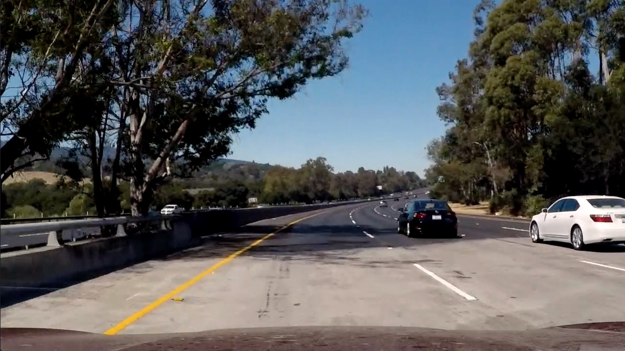
After saving the Calibration parameters in the camera calibration phase, they can be used here to undistort images using cv2.undistort() and here is the result:

This is almost the most important part in the pipeline as it filters out unimportant colors as well as pixels which are most probably not lane lines. This is done by transforming the RGB image to HSL color space and to grayscale image. A gradient threshold(thresh_gradient() in 4th cell) is done on both new images and then they are merged to form the binary image. The last step is to mask this image to process only the region of interests(directly infront of the car where the lane would be). This part can be found in the 5th cell inmain/Lane Detection.ipynb. The result is shown below:

The code for perspective transform is included in perspective_transform() in the 4th cell in main/Lane Detection.ipynb. it is a wrapper for opencv functions getPerspectiveTransform() and warpPerspective() The source and destination points are calculated as follow:

p1 = [int(0.2*shape[1]),shape[0]]
p2 = [int(0.46*shape[1]),int(0.66*shape[0])]
p3 = [int(0.625*shape[1]),int(0.66*shape[0])]
p4 = [int(0.9*shape[1]),shape[0]]
src = np.float32([p1,p2,p3,p4])
#destination points
p1 = [int(0.27*shape[1]),shape[0]]
p2 = [int(0.33*shape[1]),0]
p3 = [int(0.83*shape[1]),0]
p4 = [int(0.7*shape[1]),shape[0]]

The result of perspective transform is shown below:

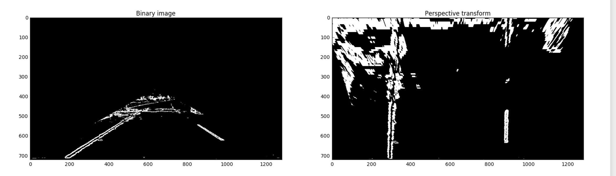
It's clear that the perspective transfrom is working correctly as the line boundaries are parallel, however there is some noise due to shadow.

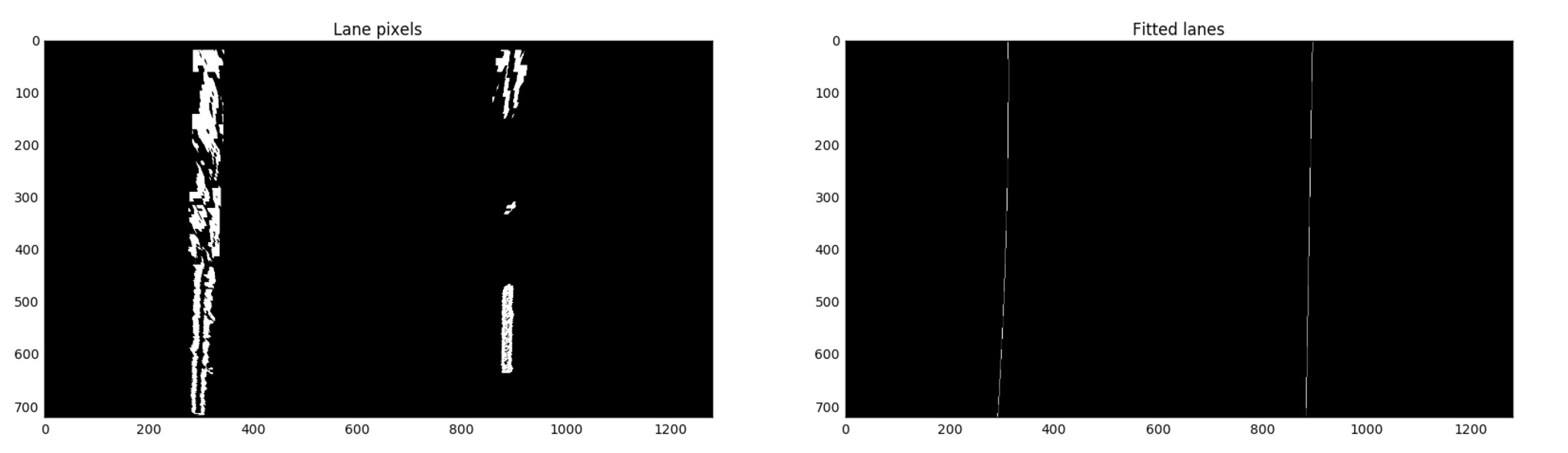
Identifying lane pixels is defined in the function find_lane_pixels() in the 4th cell in main/Lane Detection.ipynb. To get the starting point of each lane I used a histogram for the lower half of the image then used a sliding window approach to detect the rest of the points going upwards to the top of the image, I chose the window size to be 50X60 which gave great results. Here is the result of finding the lane pixels of the example image used for this writeup

The Lane lines are fitted in fit_lanes() in the 4th cell in main/Lane Detection.ipynb. The lane pixels detected in the last step are fitted with a 2nd order polynomial using np.polyfit(). If lines are detected the lane curvature is calcualated in the same function by fitting a polynomial(in the world space) and applying the following equation to calculate the curvature. left_curverad = ((1 + (2*left_fit_cr[0]*imshape[0]*ym_per_pix + left_fit_cr[1])**2)**1.5) / np.absolute(2*left_fit_cr[0]) The position of the car relative to the center is calculated as follows:

xm_per_pix = 3.7/(0.546875*imshape[1]) # meters per pixel in x dimension
screen_center_x = imshape[1]/2.0
lane_width_pix = np.mean(np.subtract(rightfitX,leftfitX))
lane_width = lane_width_pix * xm_per_pix
car_center = np.mean(np.add(rightfitX,leftfitX)) / 2.0
dist_off_center = (car_center - screen_center_x) * xm_per_pix

And here is the result of lane fitting

The final step is to warp back the image onto the original image, show the detected area between lanes and print calculated Lane curvature(average of both lane curvatures) and position of vehicle as shown below

Here is a link to the final video

I think a vision approach alone will not provide the needeed robustness, because there might be a lot of scenarios where it is hard to detect lane lines like different lighting conditions, lots of shadows, asphalt with varying colors and hard curves. I think the pipeline can be enhanced if lane tracking is added using Kalman filter for exmaple.